SG-Lib 2027 — moving to Python
This page describes the direction for 2027, not a download. The current release is SG-Lib 5.6 (2026), a MATLAB® toolbox — see Latest Release. ClevePython lets students program in MATLAB-compatible syntax under Python too, becoming familiar with that programming style and practising it.
MATLAB is a registered trademark of The MathWorks, Inc. This ClevePython project is independent of and is not affiliated with or endorsed by MathWorks.
A first ClevePython version already runs. The complete SG-Lib 2027 is still the direction described below — but a first version of ClevePython, the MATLAB-compatible Python core, already installs via an installer on Apple Silicon Macs. It is currently in beta testing at our chair (November 2026); a public download will follow.
▶ Watch the introduction video — ClevePython & MATLAB, the basics (MTT Lecture 1) (≈ 20 min).
Three statements about the next generation:
- SG-Lib 2027 will be based on Python.
- It will remain usable from MATLAB.
- MATLAB-compatible code in Python looks like the MATLAB code of today’s SG-Lib.
Why Python from 2027 on
Developing and using the SG-Lib in Python rather than in MATLAB makes it possible to:
- choose the package release freely and independently of the MATLAB release, and adopt the newest and least buggy version immediately;
- know the package developers and contact them directly when serious bugs have to be fixed, and be informed about ongoing changes;
- integrate further packages quickly and directly, from many different developers — preferably AI networks;
- better understand, and prepare for, the coming changes brought by the agentic AI developer scene;
- choose the IDE freely (Spyder, very similar to MATLAB R2024b, or Visual Studio, or any other Python IDE);
- stay independent of an “AI agent” product that is statically integrated into an IDE and may not keep up with the speed of AI development;
- use agentic AI (Claude, ChatGPT) much better through transparent interfaces such as
curl, which allow the most recent AI API versions to be used directly; - develop processes with drastically reduced memory demand for mechanism design and everyday automation, and keep many parallel tasks alive on one machine;
- use the installed Python environment (venv) independently of the MATLAB version (3.12 for R2024b, for example);
- let AI agents such as Claude or ChatGPT use the code far more directly in everyday work;
- let AI agents such as Claude or ChatGPT implement, verify and validate new code far more directly.
As a Python library, SG-Lib thereby brings the large Python ecosystem within direct reach — as a direction for 2027, not as finished interfaces:
- 3D graphics and rendering: Blender (which also uses the Manifold library).
- Multibody dynamics simulation: PyChrono, MuJoCo, Drake, PyDy.
- CAD kernels: SolidCraft, FreeCAD, CadQuery, build123d (OpenCASCADE).
- Teaching and geometry: GeoGebra (already reachable today via
CPSplotGG). - plus the scientific Python stack (NumPy, SciPy, Trimesh, Manifold) and many more packages.
One deliberate exception: the interactive side of Simulink/Simscape — wiring models by hand in a graphical front-end — will not be reproduced in ClevePython. We expect future design to be written as code/JSON by AI agents rather than clicked together in GUIs. Coupling to existing tools and packages, by contrast, is planned.
The same part in both worlds
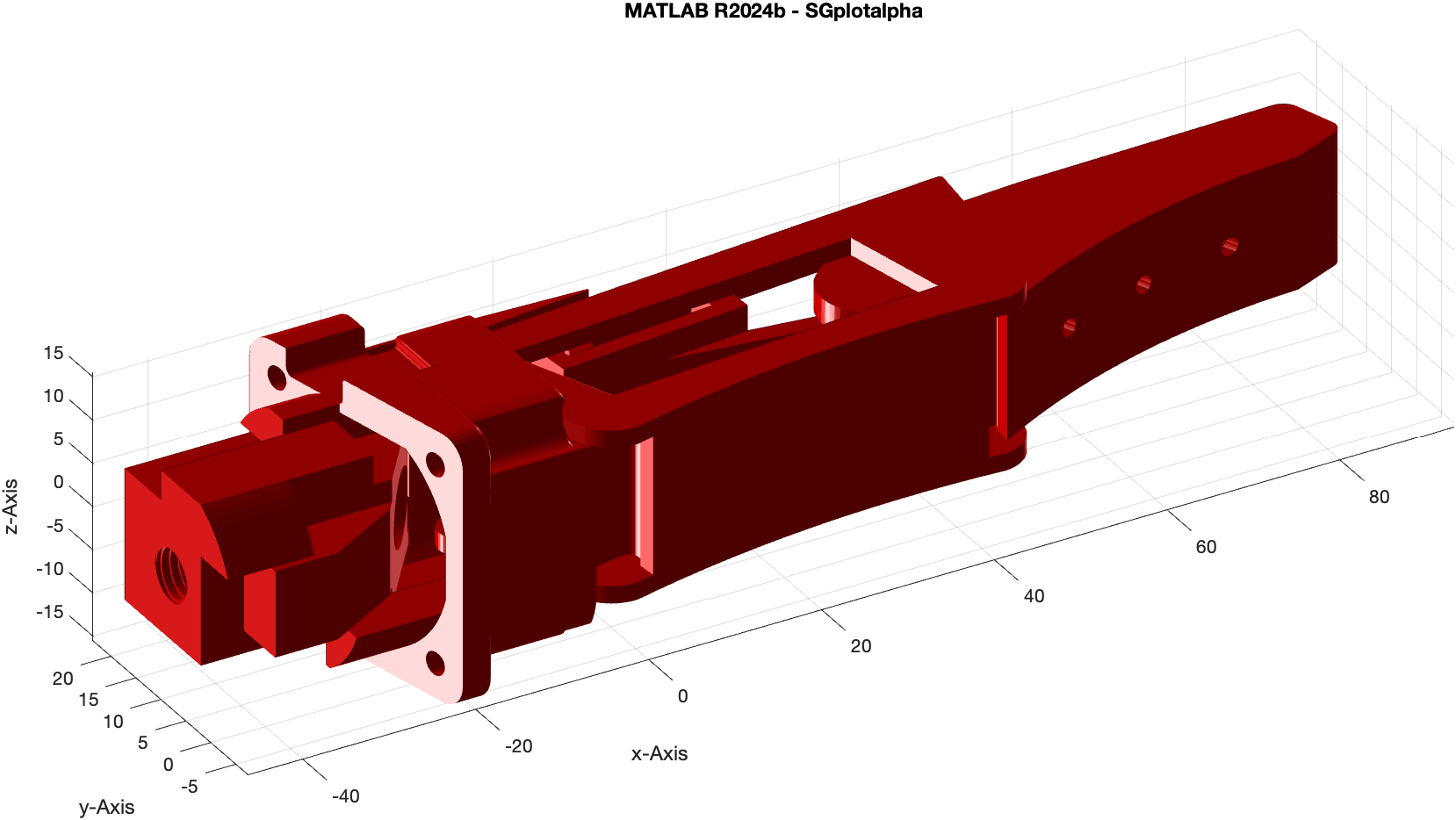
load JACO_robot.mat; SGfigure; SGplotalpha(JCF,'r'); view(-30,30)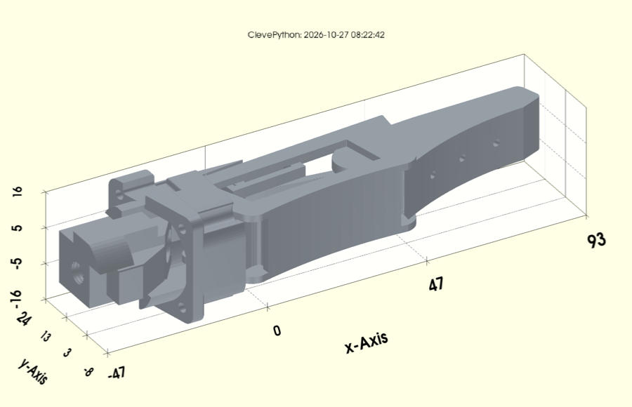
sgpyfigure that will carry SG-Lib 2027.load JACO_robot.mat; SGfigure; SGplotalpha(JCF,'r'); view(-30,30)The part is a 3D-printed finger of a JACO robot hand. The identical call in both worlds — same geometry, same viewpoint, even the same cream SG-Lib canvas — one drawn by MATLAB, one by the Python window that will carry SG-Lib 2027.
What this means for memory
The real difference is architectural. MATLAB is one process: JVM, toolboxes, graphics and workspace all together — about 1.5 GB before the first computation. The Python world is two processes: a small compute process plus a separate window. The window can be closed and restarted without losing the workspace; in MATLAB both hang on the same process.
| Process | Resident memory |
|---|---|
| Python, bare interpreter | 9 MB |
| Python with the MATLAB core and the SG-Lib functions | 70 MB |
| … with the test geometry loaded | 201 MB |
| Python graphics window with that geometry | 518 MB |
| Python total: computing + window | 719 MB |
| MATLAB, freshly started, headless | 1 473 MB |
| MATLAB desktop with graphics | 4 490 MB |
In practice: five parallel MATLAB pool workers cost about 8.7 GB today. Five Python compute processes cost about 350 MB — and they share one window.
Measured on 2026-10-27 with MATLAB R2024b on a Mac Studio (M4 Max, 128 GB, macOS 15.8.1); test geometry a 3D-printed JACO finger, 64 199 facets. Resident set size as reported by the operating system.
What this means for speed
Geometric buffering — offsetting a closed contour outward or inward — is a good test case. MATLAB’s native route is polyshape(polybuffer(CPL)), through the polybuffer and polyshape classes. SG-Lib’s CPLloopbuffer is a purely numerical re-implementation of the same operation: it uses no MATLAB classes (polybuffer/polyshape) and no geometry package (Clipper, Shapely or similar) — only arithmetic on the point list. That is what lets it preserve the start point, the winding direction and collinear points, and return the index information (which output point came from which input or auxiliary point) that the class-based route discards.
Because the algorithm is plain numerics, it ports to Python directly — and the pure-Python port is already faster than the MATLAB code. With Cython parallelization it is faster still, so the Python path wins even while keeping the collinear points and the index features that the polyshape/polybuffer route does not offer.
On an Apple M3 Pro, without 'miter' and without graphics:
| Points | Offset | MATLAB .m [ms] | Python .py [ms] | Python + Cython [ms] | polyshape + polybuffer [ms] |
|---|---|---|---|---|---|
| 12 | −1 | 1.83 | 1.42 | 0.81 | 3.13 |
| 12 | −2.5 | 13.40 | 3.25 | 2.28 | 3.25 |
| 12 | −4 | 9.41 | 3.86 | 2.97 | 1.55 |
| 12 | +4 | 0.36 | 1.42 | 0.83 | 0.67 |
| 105 | −1 | 86.03 | 17.13 | 2.60 | 1.81 |
| 105 | −2.5 | 93.92 | 18.85 | 3.04 | 2.37 |
| 105 | −4 | 93.03 | 19.65 | 3.37 | 0.95 |
| 105 | +4 | 85.21 | 17.44 | 1.28 | 0.82 |
12 points: CPLsample(3); 105 points: additionally 'aux',1.
Read the right-hand column with care. polyshape(polybuffer(…)) removes the collinear points (Simplify=true, KeepCollinearPoints=false): at 105 points it therefore buffers only 12 of the 105 points and returns no index information. CPLloopbuffer processes all 105 points and assigns each one correctly — every auxiliary point kept, with its mapping. The right-hand times at 105 points are thus the cost of a reduced 12-point problem, not of the same task.
Python and Cython were re-measured together; the MATLAB and polyshape values come from the immediately preceding comparison with unchanged MATLAB code.